Top 20 Statistics Interview Questions for Data Science

In data science, a strong foundation in statistics is essential. Learning statistical concepts can set you apart in interviews and on the job. In this blog, we’ve compiled the top 20 data science statistics interview questions to help you prepare for your next interview.

From basic concepts to advanced techniques, these questions will not only test your knowledge but also enhance your understanding of key statistical principles. So, let’s begin and get you ready to ace that interview!

Top 20 Statistics Interview Questions for Data Science

Here is a list of the top 20 statistics interview questions for data science, along with detailed explanations. 

1. Basic Statistical Concepts

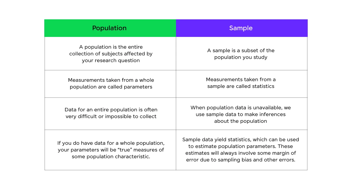
Q1: What’s the difference between population and sample? Why is this distinction important in data science?

A population refers to the entire group of individuals or items under study, while a sample is a subset of that population. This distinction is important in data science because:

1. Practicality: It’s often impossible or impractical to study an entire population.
2. Cost-effectiveness: Sampling reduces the time and resources required for data collection and analysis.
3. Inference: Proper sampling allows us to make inferences about the population based on the sample.
4. Statistical techniques: Many statistical methods are designed for sample data and include ways to account for sampling error.

Understanding this difference helps data scientists choose appropriate methods and interpret results correctly.

Q2: Explain the concepts of mean, median, and mode. When would you use each?

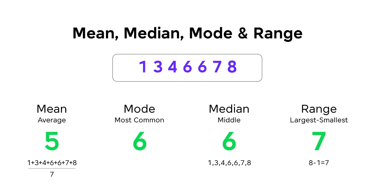
Mean: The average of a set of values, calculated by summing all values and dividing by the number of values. 

Median: The middle value when the data is ordered from lowest to highest. 

Mode: The most frequently occurring value in a dataset.

Use cases:

• Mean: Best for normally distributed data without extreme outliers. It’s useful for continuous data and when you need to account for all values in the dataset.
• Median: Preferred for skewed distributions or when there are extreme outliers. It’s often used for income data or house prices.
• Mode: Useful for categorical data or when you want to find the most common value. It’s frequently used in marketing to identify the most popular product.

Before we move into the next section, ensure you have a good grip on data science essentials like Python, MongoDB, Pandas, NumPy, Tableau & PowerBI Data Methods. If you are looking for a detailed course on Data Science, you can join GUVI’s Data Science Course with Placement Assistance. You’ll also learn about the trending tools and technologies and work on some real-time projects.  

Additionally, if you want to explore Python through a self-paced course, try GUVI’s Python course.

2. Probability Theory

Q3: What is Bayes’ Theorem, and how is it applied in data science?

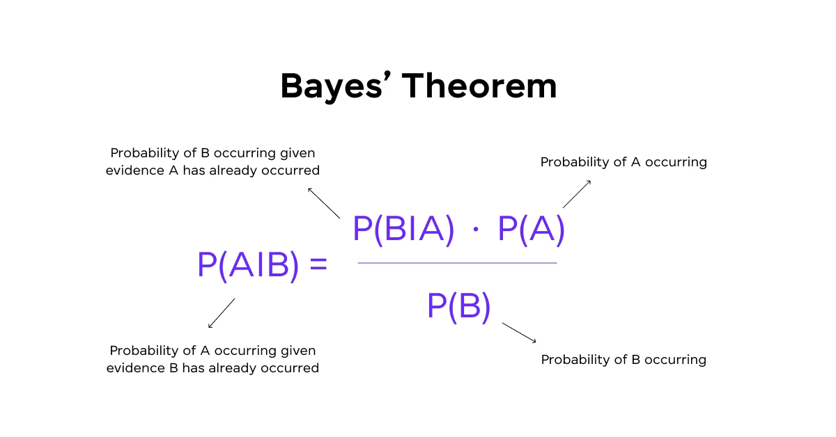
Bayes’ Theorem is a fundamental concept in probability theory that describes the probability of an event based on prior knowledge of conditions that might be related to the event. Mathematically, it’s expressed as:

P(A|B) = P(B|A) * P(A) / P(B)

Where: P(A|B) is the probability of A given B, P(B|A) is the probability of B given A, P(A) and P(B) are the probabilities of A and B independently

In data science, Bayes’ Theorem is applied in various ways:

1. Naive Bayes classifiers for text classification and spam filtering
2. Bayesian inference in A/B testing
3. Probabilistic statistical programming and modeling
4. Updating beliefs based on new evidence in machine learning models

Q4: Explain the concept of conditional probability and provide an example.

Conditional probability is the probability of an event occurring given that another event has already occurred. It’s denoted as P(A|B), read as “the probability of A given B.”

Example: In a deck of 52 cards, what’s the probability of drawing a king given that you’ve drawn a face card?

P(King | Face Card) = P(King and Face Card) / P(Face Card) = (4/52) / (12/52) = 1/3

There are 4 kings in a deck, and 12 face cards (4 each of kings, queens, and jacks). The probability of drawing a king given it’s a face card is 1/3.

3. Distributions

Q5: What is a normal distribution, and why is it important in data science?

A normal distribution, also known as a Gaussian distribution or bell curve, is a symmetric probability distribution where data near the mean is more frequent than data far from the mean. It’s characterized by its mean (μ) and standard deviation (σ).

Importance in data science:

1. Central Limit Theorem: As sample size increases, the distribution of sample means approximates a normal distribution.
2. Statistical inference: Many statistical tests assume normally distributed data.
3. Natural phenomena: Many real-world phenomena follow approximately normal distributions.
4. Machine learning: Some algorithms assume normally distributed data or errors.
5. Simplifies calculations: Properties of normal distributions make certain statistical calculations easier.

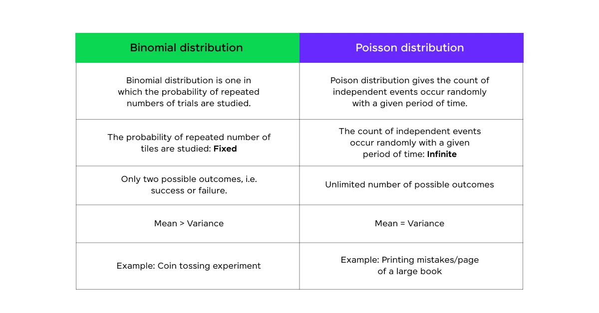
Q6: Describe the differences between a binomial distribution and a Poisson distribution.

Binomial Distribution:

• Models the number of successes in a fixed number of independent Bernoulli trials.
• Has two parameters: n (number of trials) and p (probability of success).
• Mean = np, Variance = np(1-p)
• Example: Number of heads in 10 coin flips.

Poisson Distribution:

• Models the number of events occurring in a fixed interval of time or space.
• Has one parameter: λ (average rate of occurrence)
• Mean = Variance = λ
• Example: Number of customers arriving at a store in an hour.

Key differences:

1. Binomial has a fixed number of trials, while Poisson doesn’t.
2. Binomial events are dependent (limited by n), while Poisson events are independent.
3. Binomial probabilities sum to 1, while Poisson is unbounded.

4. Hypothesis Testing

Q7: Explain the concept of p-value and its role in hypothesis testing.

The p-value is the probability of obtaining test results at least as extreme as the observed results, assuming that the null hypothesis is true. In other words, it quantifies the strength of evidence against the null hypothesis.

Role in hypothesis testing:

1. Decision making: Comparing the p-value to a predetermined significance level (usually 0.05) helps decide whether to reject the null hypothesis.
2. Strength of evidence: Smaller p-values indicate stronger evidence against the null hypothesis.
3. Continuous measure: Unlike a simple yes/no decision, p-values provide a continuous measure of evidence.
4. Reproducibility: P-values help assess the reproducibility of results.

It’s important to note that p-values don’t measure the size of an effect or the importance of a result. They are just one tool in the broader context of scientific inference.

Q8: What is the difference between Type I and Type II errors?

Type I Error (False Positive):

• Rejecting the null hypothesis when it’s actually true.
• Probability = α (significance level)
• Example: Convicting an innocent person in a trial.

Type II Error (False Negative):

• Failing to reject the null hypothesis when it’s actually false.
• Probability = β
• Example: Failing to detect a disease when it’s present.

Key differences:

1. Nature of error: Type I is about incorrectly claiming an effect exists, while Type II is about failing to detect an existing effect.
2. Relationship to power: Power of a test (1 – β) is related to Type II error, not Type I.
3. Control: We directly control the Type I error rate by setting α, while Type II error rate depends on sample size, effect size, and α.

Understanding both types of errors is important for designing experiments and interpreting results in data science.

5. Regression Analysis

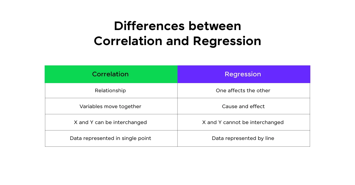
Q9: What is the difference between correlation and regression?

Correlation:

• Measures the strength and direction of a linear relationship between two variables.
• Ranges from -1 to 1, where -1 is perfect negative correlation, 0 is no correlation, and 1 is perfect positive correlation.
• Doesn’t imply causation.
• Symmetric: correlation between X and Y is the same as between Y and X.

Regression:

• Models the relationship between a dependent variable and one or more independent variables.
• Predicts the value of the dependent variable based on the independent variable(s).
• Can be used to infer causality under certain conditions.
• Asymmetric: regression of Y on X is different from X on Y.

While correlation tells us about the strength of a relationship, regression provides a mathematical equation to predict one variable from another.

Q10: Explain the assumptions of linear regression and how to check them.

Linear regression has several key assumptions:

1. Linearity: The relationship between X and Y is linear. Check: Scatter plots, residual plots.
2. Independence: Observations are independent of each other. Check: Durbin-Watson test, plot residuals against time/order.
3. Homoscedasticity: Constant variance of residuals. Check: Residual plots, Breusch-Pagan test.
4. Normality: Residuals are normally distributed. Check: Q-Q plots, histogram of residuals, Shapiro-Wilk test.
5. No multicollinearity: Independent variables are not highly correlated with each other. Check: Correlation matrix, Variance Inflation Factor (VIF).
6. No influential outliers: No single point has an undue influence on the model. Check: Cook’s distance, use plots.

Checking these assumptions are important for ensuring the validity of your linear regression model and the reliability of its predictions.

6. Data Analysis Techniques

Q11: What is the purpose of dimensionality reduction, and name two common techniques.

Dimensionality reduction is the process of reducing the number of features in a dataset while retaining as much important information as possible. Its purposes include:

1. Mitigating the curse of dimensionality
2. Reducing computational complexity
3. Removing multicollinearity
4. Improving visualization
5. Noise reduction

Two common techniques are:

1. Principal Component Analysis (PCA):
   • Linear technique that finds orthogonal axes (principal components) that capture the most variance in the data.
   • Used for continuous data.
   • Preserves global structure.
     
2. t-SNE (t-Distributed Stochastic Neighbor Embedding):
   • Non-linear technique that’s particularly good at preserving local structure.
   • Often used for visualization of high-dimensional data.
   • Better at revealing clusters or patterns in the data.

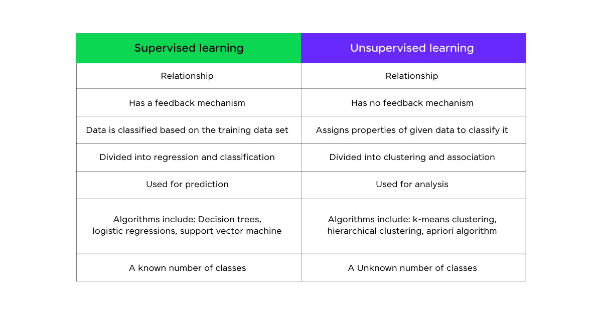
Q12: Explain the difference between supervised and unsupervised learning. Provide examples of each.

Supervised Learning:

• Involves learning a function that maps input data to known output labels.
• Requires labeled training data.
• Goal is to make accurate predictions on new, unseen data.
• Examples:
  1. Linear Regression
  2. Logistic Regression
  3. Decision Trees
  4. Support Vector Machines
  5. Neural Networks (when used for classification or regression)

Unsupervised Learning:

• Involves finding patterns or structures in data without predefined labels.
• Works with unlabeled data.
• Goal is to discover hidden patterns or groupings in data.
• Examples:
  1. K-means Clustering
  2. Hierarchical Clustering
  3. Principal Component Analysis
  4. Autoencoders
  5. Generative Adversarial Networks

The key difference is that supervised learning works towards a specific prediction task with known outcomes, while unsupervised learning explores the inherent structure of the data without predefined targets.

7. Advanced Topics

Q13: What is the bootstrap method, and how is it used in statistics?

The bootstrap method is a resampling technique used to estimate statistics on a population by sampling a dataset with replacement. It’s particularly useful when the underlying distribution is unknown or complex.

How it’s used:

1. Confidence Intervals: Estimate confidence intervals for population parameters.
2. Standard Errors: Compute standard errors of complex estimators.
3. Hypothesis Testing: Perform hypothesis tests without assuming a specific distribution.
4. Model Validation: Assess the stability and reliability of machine learning models.

Process:

1. Take a sample from the original dataset with a replacement.
2. Calculate the statistic of interest on this sample.
3. Repeat steps 1-2 many times (typically 1000+ times).
4. Use the distribution of the calculated statistics to make inferences.

The bootstrap method is powerful because it allows for inference about population parameters without making strong distributional assumptions.

Q14: Explain the concept of regularization in machine learning. What are L1 and L2 regularization?

Regularization is a technique used to prevent overfitting in machine learning models by adding a penalty term to the loss function. It discourages the model from fitting the noise in the training data too closely.

L1 Regularization (Lasso):

• Adds the absolute value of the coefficients to the loss function.
• Tends to produce sparse models by driving some coefficients to exactly zero.
• Useful for feature selection.
• Loss function: L(θ) + λ Σ|θi|

L2 Regularization (Ridge):

• Adds the squared value of the coefficients to the loss function.
• Tends to shrink coefficients towards zero, but not exactly to zero.
• Often preferred when you want to keep all features but with smaller coefficients.
• Loss function: L(θ) + λ Σθi^2

Where L(θ) is the original loss function, θi are the model parameters, and λ is the regularization strength.

Both L1 and L2 help prevent overfitting, but they have different effects on the model’s coefficients and are chosen based on the specific needs of the problem at hand.

Q15: What is the bias-variance tradeoff?

The bias-variance tradeoff is a fundamental concept in machine learning that describes the balance between two types of error that occur in model fitting:

Bias: The error introduced by approximating a real-world problem with a simplified model. High bias can lead to underfitting.

Variance: The error introduced by the model’s sensitivity to small fluctuations in the training set. High variance can lead to overfitting.

The tradeoff:

• As model complexity increases, bias tends to decrease but variance tends to increase.
• As model complexity decreases, bias tends to increase but variance tends to decrease.

The goal is to find the sweet spot that minimizes total error (bias + variance). This often involves techniques like:

1. Cross-validation
2. Regularization
3. Ensemble methods

Understanding this tradeoff helps data scientists choose appropriate model complexities and avoid both underfitting and overfitting.

Q16: Explain the concept of Maximum Likelihood Estimation (MLE).

Maximum Likelihood Estimation (MLE) is a method of estimating the parameters of a statistical model given observations. It selects the parameter values that maximize the likelihood function, which is the probability of observing the given data under the model.

Key points:

1. Goal: Find parameters that make the observed data most probable.
2. Likelihood function: L(θ|x) = P(x|θ), where θ are the parameters and x is the observed data.
3. Often work with log-likelihood for computational convenience.
4. MLE has desirable properties: consistency, efficiency, and asymptotic normality under certain conditions.

Steps:

1. Write the likelihood function based on the probability distribution.
2. Take the logarithm of the likelihood function.
3. Find the maximum by taking derivatives with respect to parameters and setting them to zero.
4. Solve the resulting equations.

MLE is widely used in statistics and machine learning for parameter estimation in various models, including linear regression, logistic regression, and many probabilistic models.

Q17: What is a confidence interval, and how is it interpreted?

A confidence interval is a range of values that is likely to contain the true population parameter with a certain level of confidence. It quantifies the uncertainty associated with a sample estimate.

Key components:

1. Point estimate: The sample statistic (e.g., sample mean)
2. Margin of error: The range around the point estimate
3. Confidence level: Usually expressed as a percentage (e.g., 95%)

Interpretation: A 95% confidence interval means that if we were to repeat the sampling process many times and calculate the confidence interval each time, about 95% of these intervals would contain the true population parameter.

Common misinterpretation: It does NOT mean there’s a 95% probability that the true parameter lies within the specific interval calculated from our sample.

Example: If a 95% CI for the population mean is [10, 12], we say: “We are 95% confident that the true population mean falls between 10 and 12.”

Understanding confidence intervals is important for making inferences about populations based on sample data in data science and statistics.

Q18: Explain the concept of statistical power and its importance in experimental design.

Statistical power is the probability that a statistical test will correctly reject the null hypothesis when it is false. In other words, it’s the likelihood of detecting an effect when it actually exists.

Power = 1 – β, where β is the probability of a Type II error (false negative).

Factors affecting power:

1. Effect size: Larger effects are easier to detect.
2. Sample size: Larger samples increase power.
3. Significance level (α): Stricter significance levels reduce power.
4. Variability in the data: Less variability increases power.

Importance in experimental design:

1. Sample size determination: Helps calculate the required sample size to detect an effect of a given size.
2. Balancing Type I and Type II errors: Allows researchers to control both false positives and false negatives.
3. Resource allocation: Ensures efficient use of resources by avoiding underpowered studies.
4. Interpretation of results: Helps interpret non-significant results (Was the effect truly absent, or was the study underpowered?).

Q19: What is the difference between parametric and non-parametric statistical methods?

Parametric Methods:

• Assume that the data follows a specific probability distribution (often normal).
• Estimate parameters of the assumed distribution from the data.
• Examples: t-test, ANOVA, linear regression.

Non-parametric Methods:

• Do not assume a specific underlying distribution.
• Often based on ranks or order statistics.
• Examples: Mann-Whitney U test, Kruskal-Wallis test, Spearman’s rank correlation.

Key differences:

1. Assumptions: Parametric methods make stronger assumptions about the data distribution.
2. Efficiency: Parametric methods are more efficient (require less data) when assumptions are met.
3. Robustness: Non-parametric methods are more robust to outliers and work better with non-normal data.
4. Interpretability: Parametric methods often provide more easily interpretable results.

Choosing between parametric and non-parametric methods depends on the nature of your data and the validity of distributional assumptions. Non-parametric methods are often preferred when dealing with small sample sizes or when the data clearly violates normality assumptions.

Q20: Explain the concept of cross-validation and its importance in model evaluation.

Cross-validation is a resampling technique used to assess how well a model will generalize to an independent dataset. It helps to detect overfitting and provides a more robust estimate of model performance than a single train-test split.

Common types of cross-validation:

1. K-Fold Cross-Validation:
   • Data is divided into k subsets.
   • Model is trained on k-1 subsets and tested on the remaining subset.
   • Process is repeated k times, with each subset serving as the test set once.
   • Results are averaged to get the overall performance.
     
2. Leave-One-Out Cross-Validation (LOOCV):
   • Special case of k-fold where k equals the number of observations.
   • Each observation serves as the test set once.
     
3. Stratified K-Fold:
   • Ensures that the proportion of samples for each class is roughly the same in each fold.
   • Useful for imbalanced datasets.

Importance in model evaluation:

1. Reduced overfitting: By testing on multiple subsets, it gives a more realistic estimate of model performance on unseen data.
2. More reliable performance estimates: Averages performance across multiple splits, reducing the impact of data partitioning.
3. Model selection: Helps in choosing between different models or hyperparameters.
4. Efficient use of data: Allows for model evaluation even with limited data.
5. Detecting data leakage: Can help identify if information from the test set is inadvertently used in training.

Cross-validation is an important technique in the data scientist’s toolkit for building robust and generalizable models.

Kickstart your Data Science journey by enrolling in GUVI’s Data Science Course where you will master technologies like MongoDB, Tableau, PowerBI, Pandas, etc., and build interesting real-life projects.

Alternatively, if you would like to explore Python through a Self-paced course, try GUVI’s Python course.

Conclusion

Learning these 20 key statistical concepts and techniques is important for success in data science interviews and real-world data analysis tasks. From fundamental concepts like probability for data science and distributions to advanced topics like regularization and cross-validation, this knowledge forms the backbone of data science practice.

Remember that while knowing these concepts is important, being able to apply them in context and explain their relevance to real-world problems is equally important. As you prepare for your data science interviews, try to think about how each of these concepts might be applied to solve actual business or research problems.

By thoroughly understanding these statistical concepts and their applications in data science, you’ll be well-prepared to tackle a wide range of interview questions and real-world data challenges. Good luck with your data science journey!

FAQs

Why are statistics important in data science interviews?

Statistics are important in data science because they provide the tools and methods needed to analyze and interpret data. Understanding statistical concepts allows you to make informed decisions, identify patterns, and validate hypotheses.
In interviews, demonstrating your proficiency in statistics shows that you have the necessary skills to handle data-driven problems and contribute effectively to data science projects.

How can I best prepare for statistics interview questions in data science?

To prepare for statistics interview questions, start by reviewing key concepts such as probability, distributions, hypothesis testing, and regression analysis. Practice solving problems related to these topics and familiarize yourself with common statistical terms and techniques.
Additionally, consider taking online courses, reading relevant books, and using practice problems or mock interviews to test your knowledge and improve your confidence.

What are some common mistakes to avoid when answering statistics interview questions?

Common mistakes to avoid include:

1. Lack of clarity: Make sure you clearly explain your thought process and reasoning.
2. Overlooking assumptions: Be aware of the assumptions underlying statistical tests and methods, and mention them when appropriate.
3. Ignoring context: Apply your statistical knowledge within the context of the problem presented, showing how it relates to real-world data science scenarios.
4. Rushing through calculations: Take your time to ensure accuracy in your calculations and explanations. 

By being mindful of these pitfalls, you can provide more thoughtful and accurate responses during your interview.